Utilities for large scale climate data analysis¶

The xarrayutils.utils module contains several functions that have proven useful in several of my day to day projects with both observational and model data.

Correlation maps¶

But what about a bit more complex task? Lets find out how mixedlayer salinity and temperature correlate. For this we use xr_linregress (for which linear_trend is just a thin wrapper):

[28]:

from xarrayutils.utils import linear_trend, xr_linregress

[29]:

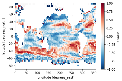
tempxsalt = xr_linregress(ds.mlt, ds.mls, dim='time')

[30]:

tempxsalt.r_value.plot()

[30]:

<matplotlib.collections.QuadMesh at 0x7f18a6857700>

This works in any dimension the dataset has:

[31]:

tempxsalt = xr_linregress(ds.mlt, ds.mls, dim='lon')

/srv/conda/envs/notebook/lib/python3.8/site-packages/xarray/core/computation.py:724: RuntimeWarning: invalid value encountered in sqrt
  result_data = func(*input_data)

[32]:

tempxsalt.r_value.plot(x='time')

[32]:

<matplotlib.collections.QuadMesh at 0x7f18a5a87850>

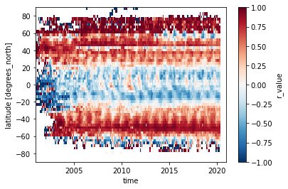
This map shows that in lower latitudes spatial patterns of salinity are generally anticorrlated with temperature and vice versa in the high latitudes.

Hatch sign agreement¶

It can often be useful to indicate if the sign along an averaged (or otherwise aggregated) dimension. For instance to show if forced changes have a consistent sign in reference to a multi-member mean. sign_agreement makes this easy. Consider this synthetic example:

[33]:

x = np.linspace(-np.pi, np.pi, 25)
y = np.linspace(-np.pi, np.pi, 25)
xx, yy = np.meshgrid(x,y)

data1 = np.sin(xx)
data2 = np.sin(yy)
data3 = np.ones_like(xx)

np.fill_diagonal(data3,np.nan)
np.fill_diagonal(data3[1:],np.nan)
np.fill_diagonal(data3[:,1:],np.nan)
np.fill_diagonal(data3[:,2:],np.nan)

da = xr.DataArray(np.array([data1, data2, data3]), dims=['member','x', 'y'])

da.plot(col='member')

[33]:

<xarray.plot.facetgrid.FacetGrid at 0x7f18a651b4f0>

Taking the mean of these fields, suggests that values increase in the upper-left, upper-right, lower-right quadrant, and the missing values in the third layer distort the mean.

[34]:

da.mean('member').plot()

[34]:

<matplotlib.collections.QuadMesh at 0x7f18a6545520>

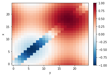
Lets produce a mask to see where all elements along the member dimension have the same sign:

[35]:

from xarrayutils.utils import sign_agreement

sign_agreement(da, da.mean('member'), 'member', threshold=1.0).plot()

[35]:

<matplotlib.collections.QuadMesh at 0x7f18a6172940>

You could use this information to indicate the areas of the average, where the members do not agree by hatching:

[36]:

da.mean('member').plot()
sign_agreement(
    da, da.mean('member'), 'member'
).plot.contourf(
    colors='none',
    hatches=['..', None],
    levels=[0,0.5],
    add_colorbar=False
)

[36]:

<matplotlib.contour.QuadContourSet at 0x7f18a66cb2b0>

Masking values in the mixed layer¶

Sometimes it is helpful to analyze data by excluding the values in the mixed layer. This can be easily done with mask_mixedlayer. Let’s see how:

First load a CMIP6 dataset from the cloud

[37]:

import intake
url = "https://raw.githubusercontent.com/NCAR/intake-esm-datastore/master/catalogs/pangeo-cmip6.json"
col = intake.open_esm_datastore(url)
cat = col.search(
    table_id='Omon',
    grid_label='gn',
    experiment_id='historical',
    member_id='r1i1p1f1',
    variable_id=['thetao','mlotst'],#,
    source_id=["ACCESS-ESM1-5"]
)
ddict = cat.to_dataset_dict(
    zarr_kwargs={'consolidated':True, 'decode_times':True},
)


--> The keys in the returned dictionary of datasets are constructed as follows:
        'activity_id.institution_id.source_id.experiment_id.table_id.grid_label'

100.00% [1/1 00:00<00:00]

[38]:

ds = ddict['CMIP.CSIRO.ACCESS-ESM1-5.historical.Omon.gn']
ds

[38]:

<xarray.Dataset>
Dimensions:             (bnds: 2, i: 360, j: 300, lev: 50, member_id: 1, time: 1980, vertices: 4)
Coordinates:
  * i                   (i) int32 0 1 2 3 4 5 6 ... 353 354 355 356 357 358 359
  * j                   (j) int32 0 1 2 3 4 5 6 ... 293 294 295 296 297 298 299
    latitude            (j, i) float64 dask.array<chunksize=(300, 360), meta=np.ndarray>
    longitude           (j, i) float64 dask.array<chunksize=(300, 360), meta=np.ndarray>
  * time                (time) datetime64[ns] 1850-01-16T12:00:00 ... 2014-12...
    time_bnds           (time, bnds) datetime64[ns] dask.array<chunksize=(1980, 2), meta=np.ndarray>
  * member_id           (member_id) <U8 'r1i1p1f1'
  * lev                 (lev) float64 5.0 15.0 25.0 ... 5.499e+03 5.831e+03
    lev_bnds            (lev, bnds) float64 dask.array<chunksize=(50, 2), meta=np.ndarray>
Dimensions without coordinates: bnds, vertices
Data variables:
    mlotst              (member_id, time, j, i) float32 dask.array<chunksize=(1, 196, 300, 360), meta=np.ndarray>
    vertices_latitude   (j, i, vertices) float64 dask.array<chunksize=(300, 360, 4), meta=np.ndarray>
    vertices_longitude  (j, i, vertices) float64 dask.array<chunksize=(300, 360, 4), meta=np.ndarray>
    thetao              (member_id, time, lev, j, i) float32 dask.array<chunksize=(1, 5, 50, 300, 360), meta=np.ndarray>
Attributes:
    grid:                    native atmosphere N96 grid (145x192 latxlon)
    forcing_index:           1
    table_id:                Omon
    variant_label:           r1i1p1f1
    source:                  ACCESS-ESM1.5 (2019): \naerosol: CLASSIC (v1.0)\...
    tracking_id:             hdl:21.14100/4ca9ce2d-6374-4e22-8ad3-1a5a6dfb8fd...
    initialization_index:    1
    physics_index:           1
    run_variant:             forcing: GHG, Oz, SA, Sl, Vl, BC, OC, (GHG = CO2...
    branch_time_in_parent:   21915.0
    history:                 2019-11-15T15:38:06Z ; CMOR rewrote data to be c...
    cmor_version:            3.4.0
    grid_label:              gn
    nominal_resolution:      250 km
    intake_esm_varname:      mlotst\nthetao
    experiment_id:           historical
    realization_index:       1
    parent_activity_id:      CMIP
    sub_experiment_id:       none
    source_id:               ACCESS-ESM1-5
    branch_time_in_child:    0.0
    parent_experiment_id:    piControl
    activity_id:             CMIP
    data_specs_version:      01.00.30
    realm:                   ocean
    product:                 model-output
    Conventions:             CF-1.7 CMIP-6.2
    experiment:              all-forcing simulation of the recent past
    mip_era:                 CMIP6
    institution:             Commonwealth Scientific and Industrial Research ...
    branch_method:           standard
    frequency:               mon
    institution_id:          CSIRO
    title:                   ACCESS-ESM1-5 output prepared for CMIP6
    table_info:              Creation Date:(30 April 2019) MD5:e14f55f257ccea...
    parent_variant_label:    r1i1p1f1
    parent_mip_era:          CMIP6
    parent_time_units:       days since 0101-1-1
    further_info_url:        https://furtherinfo.es-doc.org/CMIP6.CSIRO.ACCES...
    sub_experiment:          none
    source_type:             AOGCM
    version:                 v20191115
    parent_source_id:        ACCESS-ESM1-5
    license:                 CMIP6 model data produced by CSIRO is licensed u...
    intake_esm_dataset_key:  CMIP.CSIRO.ACCESS-ESM1-5.historical.Omon.gn

xarray.Dataset

Dimensions:
- bnds: 2
- i: 360
- j: 300
- lev: 50
- member_id: 1
- time: 1980
- vertices: 4

Coordinates: (9)

i
(i)
int32
0 1 2 3 4 5 ... 355 356 357 358 359
long_name :
cell index along first dimension
units :
1
```
array([  0,   1,   2, ..., 357, 358, 359], dtype=int32)
```
j
(j)
int32
0 1 2 3 4 5 ... 295 296 297 298 299
long_name :
cell index along second dimension
units :
1
```
array([  0,   1,   2, ..., 297, 298, 299], dtype=int32)
```

latitude

(j, i)

float64

dask.array<chunksize=(300, 360), meta=np.ndarray>

bounds :: vertices_latitude
long_name :: latitude
standard_name :: latitude
units :: degrees_north

	Array	Chunk
Bytes	864.00 kB	864.00 kB
Shape	(300, 360)	(300, 360)
Count	5 Tasks	1 Chunks
Type	float64	numpy.ndarray

longitude

(j, i)

float64

dask.array<chunksize=(300, 360), meta=np.ndarray>

bounds :: vertices_longitude
long_name :: longitude
standard_name :: longitude
units :: degrees_east

	Array	Chunk
Bytes	864.00 kB	864.00 kB
Shape	(300, 360)	(300, 360)
Count	5 Tasks	1 Chunks
Type	float64	numpy.ndarray

time

(time)

datetime64[ns]

1850-01-16T12:00:00 ... 2014-12-...

axis :: T
bounds :: time_bnds
long_name :: time
standard_name :: time

array(['1850-01-16T12:00:00.000000000', '1850-02-15T00:00:00.000000000',
       '1850-03-16T12:00:00.000000000', ..., '2014-10-16T12:00:00.000000000',
       '2014-11-16T00:00:00.000000000', '2014-12-16T12:00:00.000000000'],
      dtype='datetime64[ns]')

time_bnds

(time, bnds)

datetime64[ns]

dask.array<chunksize=(1980, 2), meta=np.ndarray>

	Array	Chunk
Bytes	31.68 kB	31.68 kB
Shape	(1980, 2)	(1980, 2)
Count	5 Tasks	1 Chunks
Type	datetime64[ns]	numpy.ndarray

member_id
(member_id)
<U8
'r1i1p1f1'
```
array(['r1i1p1f1'], dtype='<U8')
```

lev

(lev)

float64

5.0 15.0 ... 5.499e+03 5.831e+03

axis :: Z
bounds :: lev_bnds
long_name :: ocean depth coordinate
positive :: down
standard_name :: depth
units :: m

array([5.000000e+00, 1.500000e+01, 2.500000e+01, 3.500000e+01, 4.500000e+01,
       5.500000e+01, 6.500000e+01, 7.500000e+01, 8.500000e+01, 9.500000e+01,
       1.050000e+02, 1.150000e+02, 1.250000e+02, 1.350000e+02, 1.450000e+02,
       1.550000e+02, 1.650000e+02, 1.750000e+02, 1.850000e+02, 1.950000e+02,
       2.050000e+02, 2.168468e+02, 2.413490e+02, 2.807807e+02, 3.432505e+02,
       4.273156e+02, 5.367156e+02, 6.654141e+02, 8.127816e+02, 9.690651e+02,
       1.130935e+03, 1.289605e+03, 1.455770e+03, 1.622926e+03, 1.801558e+03,
       1.984855e+03, 2.182905e+03, 2.388417e+03, 2.610935e+03, 2.842564e+03,
       3.092205e+03, 3.351295e+03, 3.628058e+03, 3.913264e+03, 4.214495e+03,
       4.521918e+03, 4.842566e+03, 5.166130e+03, 5.499245e+03, 5.831294e+03])

lev_bnds

(lev, bnds)

float64

dask.array<chunksize=(50, 2), meta=np.ndarray>

	Array	Chunk
Bytes	800 B	800 B
Shape	(50, 2)	(50, 2)
Count	2 Tasks	1 Chunks
Type	float64	numpy.ndarray

Data variables: (4)

mlotst

(member_id, time, j, i)

float32

dask.array<chunksize=(1, 196, 300, 360), meta=np.ndarray>

cell_measures :: area: areacello
cell_methods :: area: mean where sea time: mean
comment :: Sigma T is potential density referenced to ocean surface.
history :: 2019-11-15T15:38:05Z altered by CMOR: replaced missing value flag (-1e+20) with standard missing value (1e+20).
long_name :: Ocean Mixed Layer Thickness Defined by Sigma T
standard_name :: ocean_mixed_layer_thickness_defined_by_sigma_t
units :: m

	Array	Chunk
Bytes	855.36 MB	84.67 MB
Shape	(1, 1980, 300, 360)	(1, 196, 300, 360)
Count	23 Tasks	11 Chunks
Type	float32	numpy.ndarray

vertices_latitude

(j, i, vertices)

float64

dask.array<chunksize=(300, 360, 4), meta=np.ndarray>

units :: degrees_north

	Array	Chunk
Bytes	3.46 MB	3.46 MB
Shape	(300, 360, 4)	(300, 360, 4)
Count	5 Tasks	1 Chunks
Type	float64	numpy.ndarray

vertices_longitude

(j, i, vertices)

float64

dask.array<chunksize=(300, 360, 4), meta=np.ndarray>

units :: degrees_east

	Array	Chunk
Bytes	3.46 MB	3.46 MB
Shape	(300, 360, 4)	(300, 360, 4)
Count	5 Tasks	1 Chunks
Type	float64	numpy.ndarray

thetao

(member_id, time, lev, j, i)

float32

dask.array<chunksize=(1, 5, 50, 300, 360), meta=np.ndarray>

cell_measures :: area: areacello volume: volcello
cell_methods :: area: mean where sea time: mean
comment :: Diagnostic should be contributed even for models using conservative temperature as prognostic field.
long_name :: Sea Water Potential Temperature
standard_name :: sea_water_potential_temperature
units :: degC

	Array	Chunk
Bytes	42.77 GB	108.00 MB
Shape	(1, 1980, 50, 300, 360)	(1, 5, 50, 300, 360)
Count	793 Tasks	396 Chunks
Type	float32	numpy.ndarray

Attributes: (45)
grid :
native atmosphere N96 grid (145x192 latxlon)
forcing_index :
1
table_id :
Omon
variant_label :
r1i1p1f1
source :
ACCESS-ESM1.5 (2019): aerosol: CLASSIC (v1.0) atmos: HadGAM2 (r1.1, N96; 192 x 145 longitude/latitude; 38 levels; top level 39255 m) atmosChem: none land: CABLE2.4 landIce: none ocean: ACCESS-OM2 (MOM5, tripolar primarily 1deg; 360 x 300 longitude/latitude; 50 levels; top grid cell 0-10 m) ocnBgchem: WOMBAT (same grid as ocean) seaIce: CICE4.1 (same grid as ocean)
tracking_id :
hdl:21.14100/4ca9ce2d-6374-4e22-8ad3-1a5a6dfb8fde hdl:21.14100/5c349831-3686-44bd-a668-b5473685d419 hdl:21.14100/daa38aaf-a8b6-432b-8711-b8e3d73ba87f hdl:21.14100/79363e12-71ec-45ff-8ac7-5d9caaf123be hdl:21.14100/a0ac1b51-fd2a-49b3-ac10-cf7f1afeb09c hdl:21.14100/33ea2626-c182-4510-924f-833bfa6efada hdl:21.14100/20e5ecb1-cbe8-438f-945e-762dfbef1caf hdl:21.14100/115a1ec8-d7c7-44d0-ae29-860faf8daea8 hdl:21.14100/d85fa960-37cc-439f-ad46-acb60581b568 hdl:21.14100/da6b29c5-d498-456f-ac04-63d595d7721e hdl:21.14100/47712943-793d-45ab-acca-b62678bce71b hdl:21.14100/1a06ae50-aac9-4e42-bf90-365ecffa0fd6 hdl:21.14100/42c2ee1a-2dc2-4976-a781-e9ce77da01c1 hdl:21.14100/19003e14-c05a-42bc-87e2-697106b55748 hdl:21.14100/2d3419d6-fc7c-4d65-9e90-ae36411f6627 hdl:21.14100/b292c680-e324-487d-89af-5e95579a6adf hdl:21.14100/5533bdc5-d82b-48ec-acd2-d4f07903f67c hdl:21.14100/c26507e7-0f70-402c-9f87-741919c26350
initialization_index :
1
physics_index :
1
run_variant :
forcing: GHG, Oz, SA, Sl, Vl, BC, OC, (GHG = CO2, N2O, CH4, CFC11, CFC12, CFC113, HCFC22, HFC125, HFC134a)
branch_time_in_parent :
21915.0
history :
2019-11-15T15:38:06Z ; CMOR rewrote data to be consistent with CMIP6, CF-1.7 CMIP-6.2 and CF standards. 2019-11-15T15:08:04Z ; CMOR rewrote data to be consistent with CMIP6, CF-1.7 CMIP-6.2 and CF standards.
cmor_version :
3.4.0
grid_label :
gn
nominal_resolution :
250 km
intake_esm_varname :
mlotst thetao
experiment_id :
historical
realization_index :
1
parent_activity_id :
CMIP
sub_experiment_id :
none
source_id :
ACCESS-ESM1-5
branch_time_in_child :
0.0
parent_experiment_id :
piControl
activity_id :
CMIP
data_specs_version :
01.00.30
realm :
ocean
product :
model-output
Conventions :
CF-1.7 CMIP-6.2
experiment :
all-forcing simulation of the recent past
mip_era :
CMIP6
institution :
Commonwealth Scientific and Industrial Research Organisation, Aspendale, Victoria 3195, Australia
branch_method :
standard
frequency :
mon
institution_id :
CSIRO
title :
ACCESS-ESM1-5 output prepared for CMIP6
table_info :
Creation Date:(30 April 2019) MD5:e14f55f257cceafb2523e41244962371
parent_variant_label :
r1i1p1f1
parent_mip_era :
CMIP6
parent_time_units :
days since 0101-1-1
further_info_url :
https://furtherinfo.es-doc.org/CMIP6.CSIRO.ACCESS-ESM1-5.historical.none.r1i1p1f1
sub_experiment :
none
source_type :
AOGCM
version :
v20191115
parent_source_id :
ACCESS-ESM1-5
license :
CMIP6 model data produced by CSIRO is licensed under a Creative Commons Attribution-ShareAlike 4.0 International License (https://creativecommons.org/licenses/). Consult https://pcmdi.llnl.gov/CMIP6/TermsOfUse for terms of use governing CMIP6 output, including citation requirements and proper acknowledgment. Further information about this data, including some limitations, can be found via the further_info_url (recorded as a global attribute in this file). The data producers and data providers make no warranty, either express or implied, including, but not limited to, warranties of merchantability and fitness for a particular purpose. All liabilities arising from the supply of the information (including any liability arising in negligence) are excluded to the fullest extent permitted by law.
intake_esm_dataset_key :
CMIP.CSIRO.ACCESS-ESM1-5.historical.Omon.gn

We can remove the values in the mixed layer

[39]:

from xarrayutils.utils import mask_mixedlayer
ds_wo_ml = mask_mixedlayer(ds, ds.mlotst)
ds_wo_ml

/home/jovyan/xarrayutils/xarrayutils/utils.py:805: UserWarning: Cell bounds [{z_bounds}] not found in input. Masking is performed with cell centers, which might be less accurate
  warnings.warn(

[39]:

<xarray.Dataset>
Dimensions:             (bnds: 2, i: 360, j: 300, lev: 50, member_id: 1, time: 1980, vertices: 4)
Coordinates:
  * i                   (i) int32 0 1 2 3 4 5 6 ... 353 354 355 356 357 358 359
  * j                   (j) int32 0 1 2 3 4 5 6 ... 293 294 295 296 297 298 299
    latitude            (j, i) float64 dask.array<chunksize=(300, 360), meta=np.ndarray>
    longitude           (j, i) float64 dask.array<chunksize=(300, 360), meta=np.ndarray>
  * time                (time) datetime64[ns] 1850-01-16T12:00:00 ... 2014-12...
    time_bnds           (time, bnds) datetime64[ns] dask.array<chunksize=(1980, 2), meta=np.ndarray>
  * member_id           (member_id) <U8 'r1i1p1f1'
  * lev                 (lev) float64 5.0 15.0 25.0 ... 5.499e+03 5.831e+03
    lev_bnds            (lev, bnds) float64 dask.array<chunksize=(50, 2), meta=np.ndarray>
Dimensions without coordinates: bnds, vertices
Data variables:
    mlotst              (member_id, time, j, i, lev) float32 dask.array<chunksize=(1, 196, 300, 360, 50), meta=np.ndarray>
    vertices_latitude   (j, i, vertices, lev, member_id, time) float64 dask.array<chunksize=(300, 360, 4, 50, 1, 196), meta=np.ndarray>
    vertices_longitude  (j, i, vertices, lev, member_id, time) float64 dask.array<chunksize=(300, 360, 4, 50, 1, 196), meta=np.ndarray>
    thetao              (member_id, time, lev, j, i) float32 dask.array<chunksize=(1, 5, 50, 300, 360), meta=np.ndarray>
Attributes:
    grid:                                 native atmosphere N96 grid (145x192...
    forcing_index:                        1
    table_id:                             Omon
    variant_label:                        r1i1p1f1
    source:                               ACCESS-ESM1.5 (2019): \naerosol: CL...
    tracking_id:                          hdl:21.14100/4ca9ce2d-6374-4e22-8ad...
    initialization_index:                 1
    physics_index:                        1
    run_variant:                          forcing: GHG, Oz, SA, Sl, Vl, BC, O...
    branch_time_in_parent:                21915.0
    history:                              2019-11-15T15:38:06Z ; CMOR rewrote...
    cmor_version:                         3.4.0
    grid_label:                           gn
    nominal_resolution:                   250 km
    intake_esm_varname:                   mlotst\nthetao
    experiment_id:                        historical
    realization_index:                    1
    parent_activity_id:                   CMIP
    sub_experiment_id:                    none
    source_id:                            ACCESS-ESM1-5
    branch_time_in_child:                 0.0
    parent_experiment_id:                 piControl
    activity_id:                          CMIP
    data_specs_version:                   01.00.30
    realm:                                ocean
    product:                              model-output
    Conventions:                          CF-1.7 CMIP-6.2
    experiment:                           all-forcing simulation of the recen...
    mip_era:                              CMIP6
    institution:                          Commonwealth Scientific and Industr...
    branch_method:                        standard
    frequency:                            mon
    institution_id:                       CSIRO
    title:                                ACCESS-ESM1-5 output prepared for C...
    table_info:                           Creation Date:(30 April 2019) MD5:e...
    parent_variant_label:                 r1i1p1f1
    parent_mip_era:                       CMIP6
    parent_time_units:                    days since 0101-1-1
    further_info_url:                     https://furtherinfo.es-doc.org/CMIP...
    sub_experiment:                       none
    source_type:                          AOGCM
    version:                              v20191115
    parent_source_id:                     ACCESS-ESM1-5
    license:                              CMIP6 model data produced by CSIRO ...
    intake_esm_dataset_key:               CMIP.CSIRO.ACCESS-ESM1-5.historical...
    mixed_layer_values_removed_based_on:  lev

xarray.Dataset

Dimensions:
- bnds: 2
- i: 360
- j: 300
- lev: 50
- member_id: 1
- time: 1980
- vertices: 4

Coordinates: (9)

i
(i)
int32
0 1 2 3 4 5 ... 355 356 357 358 359
long_name :
cell index along first dimension
units :
1
```
array([  0,   1,   2, ..., 357, 358, 359], dtype=int32)
```
j
(j)
int32
0 1 2 3 4 5 ... 295 296 297 298 299
long_name :
cell index along second dimension
units :
1
```
array([  0,   1,   2, ..., 297, 298, 299], dtype=int32)
```

latitude

(j, i)

float64

dask.array<chunksize=(300, 360), meta=np.ndarray>

bounds :: vertices_latitude
long_name :: latitude
standard_name :: latitude
units :: degrees_north

	Array	Chunk
Bytes	864.00 kB	864.00 kB
Shape	(300, 360)	(300, 360)
Count	5 Tasks	1 Chunks
Type	float64	numpy.ndarray

longitude

(j, i)

float64

dask.array<chunksize=(300, 360), meta=np.ndarray>

bounds :: vertices_longitude
long_name :: longitude
standard_name :: longitude
units :: degrees_east

	Array	Chunk
Bytes	864.00 kB	864.00 kB
Shape	(300, 360)	(300, 360)
Count	5 Tasks	1 Chunks
Type	float64	numpy.ndarray

time

(time)

datetime64[ns]

1850-01-16T12:00:00 ... 2014-12-...

axis :: T
bounds :: time_bnds
long_name :: time
standard_name :: time

array(['1850-01-16T12:00:00.000000000', '1850-02-15T00:00:00.000000000',
       '1850-03-16T12:00:00.000000000', ..., '2014-10-16T12:00:00.000000000',
       '2014-11-16T00:00:00.000000000', '2014-12-16T12:00:00.000000000'],
      dtype='datetime64[ns]')

time_bnds

(time, bnds)

datetime64[ns]

dask.array<chunksize=(1980, 2), meta=np.ndarray>

	Array	Chunk
Bytes	31.68 kB	31.68 kB
Shape	(1980, 2)	(1980, 2)
Count	5 Tasks	1 Chunks
Type	datetime64[ns]	numpy.ndarray

member_id
(member_id)
<U8
'r1i1p1f1'
```
array(['r1i1p1f1'], dtype='<U8')
```

lev

(lev)

float64

5.0 15.0 ... 5.499e+03 5.831e+03

axis :: Z
bounds :: lev_bnds
long_name :: ocean depth coordinate
positive :: down
standard_name :: depth
units :: m

array([5.000000e+00, 1.500000e+01, 2.500000e+01, 3.500000e+01, 4.500000e+01,
       5.500000e+01, 6.500000e+01, 7.500000e+01, 8.500000e+01, 9.500000e+01,
       1.050000e+02, 1.150000e+02, 1.250000e+02, 1.350000e+02, 1.450000e+02,
       1.550000e+02, 1.650000e+02, 1.750000e+02, 1.850000e+02, 1.950000e+02,
       2.050000e+02, 2.168468e+02, 2.413490e+02, 2.807807e+02, 3.432505e+02,
       4.273156e+02, 5.367156e+02, 6.654141e+02, 8.127816e+02, 9.690651e+02,
       1.130935e+03, 1.289605e+03, 1.455770e+03, 1.622926e+03, 1.801558e+03,
       1.984855e+03, 2.182905e+03, 2.388417e+03, 2.610935e+03, 2.842564e+03,
       3.092205e+03, 3.351295e+03, 3.628058e+03, 3.913264e+03, 4.214495e+03,
       4.521918e+03, 4.842566e+03, 5.166130e+03, 5.499245e+03, 5.831294e+03])

lev_bnds

(lev, bnds)

float64

dask.array<chunksize=(50, 2), meta=np.ndarray>

	Array	Chunk
Bytes	800 B	800 B
Shape	(50, 2)	(50, 2)
Count	2 Tasks	1 Chunks
Type	float64	numpy.ndarray

Data variables: (4)

mlotst

(member_id, time, j, i, lev)

float32

dask.array<chunksize=(1, 196, 300, 360, 50), meta=np.ndarray>

cell_measures :: area: areacello
cell_methods :: area: mean where sea time: mean
comment :: Sigma T is potential density referenced to ocean surface.
history :: 2019-11-15T15:38:05Z altered by CMOR: replaced missing value flag (-1e+20) with standard missing value (1e+20).
long_name :: Ocean Mixed Layer Thickness Defined by Sigma T
standard_name :: ocean_mixed_layer_thickness_defined_by_sigma_t
units :: m

	Array	Chunk
Bytes	42.77 GB	4.23 GB
Shape	(1, 1980, 300, 360, 50)	(1, 196, 300, 360, 50)
Count	101 Tasks	11 Chunks
Type	float32	numpy.ndarray

vertices_latitude

(j, i, vertices, lev, member_id, time)

float64

dask.array<chunksize=(300, 360, 4, 50, 1, 196), meta=np.ndarray>

units :: degrees_north

	Array	Chunk
Bytes	342.14 GB	33.87 GB
Shape	(300, 360, 4, 50, 1, 1980)	(300, 360, 4, 50, 1, 196)
Count	107 Tasks	11 Chunks
Type	float64	numpy.ndarray

vertices_longitude

(j, i, vertices, lev, member_id, time)

float64

dask.array<chunksize=(300, 360, 4, 50, 1, 196), meta=np.ndarray>

units :: degrees_east

	Array	Chunk
Bytes	342.14 GB	33.87 GB
Shape	(300, 360, 4, 50, 1, 1980)	(300, 360, 4, 50, 1, 196)
Count	107 Tasks	11 Chunks
Type	float64	numpy.ndarray

thetao

(member_id, time, lev, j, i)

float32

dask.array<chunksize=(1, 5, 50, 300, 360), meta=np.ndarray>

cell_measures :: area: areacello volume: volcello
cell_methods :: area: mean where sea time: mean
comment :: Diagnostic should be contributed even for models using conservative temperature as prognostic field.
long_name :: Sea Water Potential Temperature
standard_name :: sea_water_potential_temperature
units :: degC

	Array	Chunk
Bytes	42.77 GB	108.00 MB
Shape	(1, 1980, 50, 300, 360)	(1, 5, 50, 300, 360)
Count	2504 Tasks	404 Chunks
Type	float32	numpy.ndarray

Attributes: (46)
grid :
native atmosphere N96 grid (145x192 latxlon)
forcing_index :
1
table_id :
Omon
variant_label :
r1i1p1f1
source :
ACCESS-ESM1.5 (2019): aerosol: CLASSIC (v1.0) atmos: HadGAM2 (r1.1, N96; 192 x 145 longitude/latitude; 38 levels; top level 39255 m) atmosChem: none land: CABLE2.4 landIce: none ocean: ACCESS-OM2 (MOM5, tripolar primarily 1deg; 360 x 300 longitude/latitude; 50 levels; top grid cell 0-10 m) ocnBgchem: WOMBAT (same grid as ocean) seaIce: CICE4.1 (same grid as ocean)
tracking_id :
hdl:21.14100/4ca9ce2d-6374-4e22-8ad3-1a5a6dfb8fde hdl:21.14100/5c349831-3686-44bd-a668-b5473685d419 hdl:21.14100/daa38aaf-a8b6-432b-8711-b8e3d73ba87f hdl:21.14100/79363e12-71ec-45ff-8ac7-5d9caaf123be hdl:21.14100/a0ac1b51-fd2a-49b3-ac10-cf7f1afeb09c hdl:21.14100/33ea2626-c182-4510-924f-833bfa6efada hdl:21.14100/20e5ecb1-cbe8-438f-945e-762dfbef1caf hdl:21.14100/115a1ec8-d7c7-44d0-ae29-860faf8daea8 hdl:21.14100/d85fa960-37cc-439f-ad46-acb60581b568 hdl:21.14100/da6b29c5-d498-456f-ac04-63d595d7721e hdl:21.14100/47712943-793d-45ab-acca-b62678bce71b hdl:21.14100/1a06ae50-aac9-4e42-bf90-365ecffa0fd6 hdl:21.14100/42c2ee1a-2dc2-4976-a781-e9ce77da01c1 hdl:21.14100/19003e14-c05a-42bc-87e2-697106b55748 hdl:21.14100/2d3419d6-fc7c-4d65-9e90-ae36411f6627 hdl:21.14100/b292c680-e324-487d-89af-5e95579a6adf hdl:21.14100/5533bdc5-d82b-48ec-acd2-d4f07903f67c hdl:21.14100/c26507e7-0f70-402c-9f87-741919c26350
initialization_index :
1
physics_index :
1
run_variant :
forcing: GHG, Oz, SA, Sl, Vl, BC, OC, (GHG = CO2, N2O, CH4, CFC11, CFC12, CFC113, HCFC22, HFC125, HFC134a)
branch_time_in_parent :
21915.0
history :
2019-11-15T15:38:06Z ; CMOR rewrote data to be consistent with CMIP6, CF-1.7 CMIP-6.2 and CF standards. 2019-11-15T15:08:04Z ; CMOR rewrote data to be consistent with CMIP6, CF-1.7 CMIP-6.2 and CF standards.
cmor_version :
3.4.0
grid_label :
gn
nominal_resolution :
250 km
intake_esm_varname :
mlotst thetao
experiment_id :
historical
realization_index :
1
parent_activity_id :
CMIP
sub_experiment_id :
none
source_id :
ACCESS-ESM1-5
branch_time_in_child :
0.0
parent_experiment_id :
piControl
activity_id :
CMIP
data_specs_version :
01.00.30
realm :
ocean
product :
model-output
Conventions :
CF-1.7 CMIP-6.2
experiment :
all-forcing simulation of the recent past
mip_era :
CMIP6
institution :
Commonwealth Scientific and Industrial Research Organisation, Aspendale, Victoria 3195, Australia
branch_method :
standard
frequency :
mon
institution_id :
CSIRO
title :
ACCESS-ESM1-5 output prepared for CMIP6
table_info :
Creation Date:(30 April 2019) MD5:e14f55f257cceafb2523e41244962371
parent_variant_label :
r1i1p1f1
parent_mip_era :
CMIP6
parent_time_units :
days since 0101-1-1
further_info_url :
https://furtherinfo.es-doc.org/CMIP6.CSIRO.ACCESS-ESM1-5.historical.none.r1i1p1f1
sub_experiment :
none
source_type :
AOGCM
version :
v20191115
parent_source_id :
ACCESS-ESM1-5
license :
CMIP6 model data produced by CSIRO is licensed under a Creative Commons Attribution-ShareAlike 4.0 International License (https://creativecommons.org/licenses/). Consult https://pcmdi.llnl.gov/CMIP6/TermsOfUse for terms of use governing CMIP6 output, including citation requirements and proper acknowledgment. Further information about this data, including some limitations, can be found via the further_info_url (recorded as a global attribute in this file). The data producers and data providers make no warranty, either express or implied, including, but not limited to, warranties of merchantability and fitness for a particular purpose. All liabilities arising from the supply of the information (including any liability arising in negligence) are excluded to the fullest extent permitted by law.
intake_esm_dataset_key :
CMIP.CSIRO.ACCESS-ESM1-5.historical.Omon.gn
mixed_layer_values_removed_based_on :
lev

Or to have the mixed layer values only

[40]:

from xarrayutils.utils import mask_mixedlayer
ds_ml_only = mask_mixedlayer(ds, ds.mlotst, mask='inside')
ds_ml_only

/home/jovyan/xarrayutils/xarrayutils/utils.py:805: UserWarning: Cell bounds [{z_bounds}] not found in input. Masking is performed with cell centers, which might be less accurate
  warnings.warn(

[40]:

<xarray.Dataset>
Dimensions:             (bnds: 2, i: 360, j: 300, lev: 50, member_id: 1, time: 1980, vertices: 4)
Coordinates:
  * i                   (i) int32 0 1 2 3 4 5 6 ... 353 354 355 356 357 358 359
  * j                   (j) int32 0 1 2 3 4 5 6 ... 293 294 295 296 297 298 299
    latitude            (j, i) float64 dask.array<chunksize=(300, 360), meta=np.ndarray>
    longitude           (j, i) float64 dask.array<chunksize=(300, 360), meta=np.ndarray>
  * time                (time) datetime64[ns] 1850-01-16T12:00:00 ... 2014-12...
    time_bnds           (time, bnds) datetime64[ns] dask.array<chunksize=(1980, 2), meta=np.ndarray>
  * member_id           (member_id) <U8 'r1i1p1f1'
  * lev                 (lev) float64 5.0 15.0 25.0 ... 5.499e+03 5.831e+03
    lev_bnds            (lev, bnds) float64 dask.array<chunksize=(50, 2), meta=np.ndarray>
Dimensions without coordinates: bnds, vertices
Data variables:
    mlotst              (member_id, time, j, i, lev) float32 dask.array<chunksize=(1, 196, 300, 360, 50), meta=np.ndarray>
    vertices_latitude   (j, i, vertices, lev, member_id, time) float64 dask.array<chunksize=(300, 360, 4, 50, 1, 196), meta=np.ndarray>
    vertices_longitude  (j, i, vertices, lev, member_id, time) float64 dask.array<chunksize=(300, 360, 4, 50, 1, 196), meta=np.ndarray>
    thetao              (member_id, time, lev, j, i) float32 dask.array<chunksize=(1, 5, 50, 300, 360), meta=np.ndarray>
Attributes:
    grid:                                 native atmosphere N96 grid (145x192...
    forcing_index:                        1
    table_id:                             Omon
    variant_label:                        r1i1p1f1
    source:                               ACCESS-ESM1.5 (2019): \naerosol: CL...
    tracking_id:                          hdl:21.14100/4ca9ce2d-6374-4e22-8ad...
    initialization_index:                 1
    physics_index:                        1
    run_variant:                          forcing: GHG, Oz, SA, Sl, Vl, BC, O...
    branch_time_in_parent:                21915.0
    history:                              2019-11-15T15:38:06Z ; CMOR rewrote...
    cmor_version:                         3.4.0
    grid_label:                           gn
    nominal_resolution:                   250 km
    intake_esm_varname:                   mlotst\nthetao
    experiment_id:                        historical
    realization_index:                    1
    parent_activity_id:                   CMIP
    sub_experiment_id:                    none
    source_id:                            ACCESS-ESM1-5
    branch_time_in_child:                 0.0
    parent_experiment_id:                 piControl
    activity_id:                          CMIP
    data_specs_version:                   01.00.30
    realm:                                ocean
    product:                              model-output
    Conventions:                          CF-1.7 CMIP-6.2
    experiment:                           all-forcing simulation of the recen...
    mip_era:                              CMIP6
    institution:                          Commonwealth Scientific and Industr...
    branch_method:                        standard
    frequency:                            mon
    institution_id:                       CSIRO
    title:                                ACCESS-ESM1-5 output prepared for C...
    table_info:                           Creation Date:(30 April 2019) MD5:e...
    parent_variant_label:                 r1i1p1f1
    parent_mip_era:                       CMIP6
    parent_time_units:                    days since 0101-1-1
    further_info_url:                     https://furtherinfo.es-doc.org/CMIP...
    sub_experiment:                       none
    source_type:                          AOGCM
    version:                              v20191115
    parent_source_id:                     ACCESS-ESM1-5
    license:                              CMIP6 model data produced by CSIRO ...
    intake_esm_dataset_key:               CMIP.CSIRO.ACCESS-ESM1-5.historical...
    mixed_layer_values_removed_based_on:  lev

xarray.Dataset

Dimensions:
- bnds: 2
- i: 360
- j: 300
- lev: 50
- member_id: 1
- time: 1980
- vertices: 4

Coordinates: (9)

i
(i)
int32
0 1 2 3 4 5 ... 355 356 357 358 359
long_name :
cell index along first dimension
units :
1
```
array([  0,   1,   2, ..., 357, 358, 359], dtype=int32)
```
j
(j)
int32
0 1 2 3 4 5 ... 295 296 297 298 299
long_name :
cell index along second dimension
units :
1
```
array([  0,   1,   2, ..., 297, 298, 299], dtype=int32)
```

latitude

(j, i)

float64

dask.array<chunksize=(300, 360), meta=np.ndarray>

bounds :: vertices_latitude
long_name :: latitude
standard_name :: latitude
units :: degrees_north

	Array	Chunk
Bytes	864.00 kB	864.00 kB
Shape	(300, 360)	(300, 360)
Count	5 Tasks	1 Chunks
Type	float64	numpy.ndarray

longitude

(j, i)

float64

dask.array<chunksize=(300, 360), meta=np.ndarray>

bounds :: vertices_longitude
long_name :: longitude
standard_name :: longitude
units :: degrees_east

	Array	Chunk
Bytes	864.00 kB	864.00 kB
Shape	(300, 360)	(300, 360)
Count	5 Tasks	1 Chunks
Type	float64	numpy.ndarray

time

(time)

datetime64[ns]

1850-01-16T12:00:00 ... 2014-12-...

axis :: T
bounds :: time_bnds
long_name :: time
standard_name :: time

array(['1850-01-16T12:00:00.000000000', '1850-02-15T00:00:00.000000000',
       '1850-03-16T12:00:00.000000000', ..., '2014-10-16T12:00:00.000000000',
       '2014-11-16T00:00:00.000000000', '2014-12-16T12:00:00.000000000'],
      dtype='datetime64[ns]')

time_bnds

(time, bnds)

datetime64[ns]

dask.array<chunksize=(1980, 2), meta=np.ndarray>

	Array	Chunk
Bytes	31.68 kB	31.68 kB
Shape	(1980, 2)	(1980, 2)
Count	5 Tasks	1 Chunks
Type	datetime64[ns]	numpy.ndarray

member_id
(member_id)
<U8
'r1i1p1f1'
```
array(['r1i1p1f1'], dtype='<U8')
```

lev

(lev)

float64

5.0 15.0 ... 5.499e+03 5.831e+03

axis :: Z
bounds :: lev_bnds
long_name :: ocean depth coordinate
positive :: down
standard_name :: depth
units :: m

array([5.000000e+00, 1.500000e+01, 2.500000e+01, 3.500000e+01, 4.500000e+01,
       5.500000e+01, 6.500000e+01, 7.500000e+01, 8.500000e+01, 9.500000e+01,
       1.050000e+02, 1.150000e+02, 1.250000e+02, 1.350000e+02, 1.450000e+02,
       1.550000e+02, 1.650000e+02, 1.750000e+02, 1.850000e+02, 1.950000e+02,
       2.050000e+02, 2.168468e+02, 2.413490e+02, 2.807807e+02, 3.432505e+02,
       4.273156e+02, 5.367156e+02, 6.654141e+02, 8.127816e+02, 9.690651e+02,
       1.130935e+03, 1.289605e+03, 1.455770e+03, 1.622926e+03, 1.801558e+03,
       1.984855e+03, 2.182905e+03, 2.388417e+03, 2.610935e+03, 2.842564e+03,
       3.092205e+03, 3.351295e+03, 3.628058e+03, 3.913264e+03, 4.214495e+03,
       4.521918e+03, 4.842566e+03, 5.166130e+03, 5.499245e+03, 5.831294e+03])

lev_bnds

(lev, bnds)

float64

dask.array<chunksize=(50, 2), meta=np.ndarray>

	Array	Chunk
Bytes	800 B	800 B
Shape	(50, 2)	(50, 2)
Count	2 Tasks	1 Chunks
Type	float64	numpy.ndarray

Data variables: (4)

mlotst

(member_id, time, j, i, lev)

float32

dask.array<chunksize=(1, 196, 300, 360, 50), meta=np.ndarray>

cell_measures :: area: areacello
cell_methods :: area: mean where sea time: mean
comment :: Sigma T is potential density referenced to ocean surface.
history :: 2019-11-15T15:38:05Z altered by CMOR: replaced missing value flag (-1e+20) with standard missing value (1e+20).
long_name :: Ocean Mixed Layer Thickness Defined by Sigma T
standard_name :: ocean_mixed_layer_thickness_defined_by_sigma_t
units :: m

	Array	Chunk
Bytes	42.77 GB	4.23 GB
Shape	(1, 1980, 300, 360, 50)	(1, 196, 300, 360, 50)
Count	101 Tasks	11 Chunks
Type	float32	numpy.ndarray

vertices_latitude

(j, i, vertices, lev, member_id, time)

float64

dask.array<chunksize=(300, 360, 4, 50, 1, 196), meta=np.ndarray>

units :: degrees_north

	Array	Chunk
Bytes	342.14 GB	33.87 GB
Shape	(300, 360, 4, 50, 1, 1980)	(300, 360, 4, 50, 1, 196)
Count	107 Tasks	11 Chunks
Type	float64	numpy.ndarray

vertices_longitude

(j, i, vertices, lev, member_id, time)

float64

dask.array<chunksize=(300, 360, 4, 50, 1, 196), meta=np.ndarray>

units :: degrees_east

	Array	Chunk
Bytes	342.14 GB	33.87 GB
Shape	(300, 360, 4, 50, 1, 1980)	(300, 360, 4, 50, 1, 196)
Count	107 Tasks	11 Chunks
Type	float64	numpy.ndarray

thetao

(member_id, time, lev, j, i)

float32

dask.array<chunksize=(1, 5, 50, 300, 360), meta=np.ndarray>

cell_measures :: area: areacello volume: volcello
cell_methods :: area: mean where sea time: mean
comment :: Diagnostic should be contributed even for models using conservative temperature as prognostic field.
long_name :: Sea Water Potential Temperature
standard_name :: sea_water_potential_temperature
units :: degC

	Array	Chunk
Bytes	42.77 GB	108.00 MB
Shape	(1, 1980, 50, 300, 360)	(1, 5, 50, 300, 360)
Count	2504 Tasks	404 Chunks
Type	float32	numpy.ndarray

Attributes: (46)
grid :
native atmosphere N96 grid (145x192 latxlon)
forcing_index :
1
table_id :
Omon
variant_label :
r1i1p1f1
source :
ACCESS-ESM1.5 (2019): aerosol: CLASSIC (v1.0) atmos: HadGAM2 (r1.1, N96; 192 x 145 longitude/latitude; 38 levels; top level 39255 m) atmosChem: none land: CABLE2.4 landIce: none ocean: ACCESS-OM2 (MOM5, tripolar primarily 1deg; 360 x 300 longitude/latitude; 50 levels; top grid cell 0-10 m) ocnBgchem: WOMBAT (same grid as ocean) seaIce: CICE4.1 (same grid as ocean)
tracking_id :
hdl:21.14100/4ca9ce2d-6374-4e22-8ad3-1a5a6dfb8fde hdl:21.14100/5c349831-3686-44bd-a668-b5473685d419 hdl:21.14100/daa38aaf-a8b6-432b-8711-b8e3d73ba87f hdl:21.14100/79363e12-71ec-45ff-8ac7-5d9caaf123be hdl:21.14100/a0ac1b51-fd2a-49b3-ac10-cf7f1afeb09c hdl:21.14100/33ea2626-c182-4510-924f-833bfa6efada hdl:21.14100/20e5ecb1-cbe8-438f-945e-762dfbef1caf hdl:21.14100/115a1ec8-d7c7-44d0-ae29-860faf8daea8 hdl:21.14100/d85fa960-37cc-439f-ad46-acb60581b568 hdl:21.14100/da6b29c5-d498-456f-ac04-63d595d7721e hdl:21.14100/47712943-793d-45ab-acca-b62678bce71b hdl:21.14100/1a06ae50-aac9-4e42-bf90-365ecffa0fd6 hdl:21.14100/42c2ee1a-2dc2-4976-a781-e9ce77da01c1 hdl:21.14100/19003e14-c05a-42bc-87e2-697106b55748 hdl:21.14100/2d3419d6-fc7c-4d65-9e90-ae36411f6627 hdl:21.14100/b292c680-e324-487d-89af-5e95579a6adf hdl:21.14100/5533bdc5-d82b-48ec-acd2-d4f07903f67c hdl:21.14100/c26507e7-0f70-402c-9f87-741919c26350
initialization_index :
1
physics_index :
1
run_variant :
forcing: GHG, Oz, SA, Sl, Vl, BC, OC, (GHG = CO2, N2O, CH4, CFC11, CFC12, CFC113, HCFC22, HFC125, HFC134a)
branch_time_in_parent :
21915.0
history :
2019-11-15T15:38:06Z ; CMOR rewrote data to be consistent with CMIP6, CF-1.7 CMIP-6.2 and CF standards. 2019-11-15T15:08:04Z ; CMOR rewrote data to be consistent with CMIP6, CF-1.7 CMIP-6.2 and CF standards.
cmor_version :
3.4.0
grid_label :
gn
nominal_resolution :
250 km
intake_esm_varname :
mlotst thetao
experiment_id :
historical
realization_index :
1
parent_activity_id :
CMIP
sub_experiment_id :
none
source_id :
ACCESS-ESM1-5
branch_time_in_child :
0.0
parent_experiment_id :
piControl
activity_id :
CMIP
data_specs_version :
01.00.30
realm :
ocean
product :
model-output
Conventions :
CF-1.7 CMIP-6.2
experiment :
all-forcing simulation of the recent past
mip_era :
CMIP6
institution :
Commonwealth Scientific and Industrial Research Organisation, Aspendale, Victoria 3195, Australia
branch_method :
standard
frequency :
mon
institution_id :
CSIRO
title :
ACCESS-ESM1-5 output prepared for CMIP6
table_info :
Creation Date:(30 April 2019) MD5:e14f55f257cceafb2523e41244962371
parent_variant_label :
r1i1p1f1
parent_mip_era :
CMIP6
parent_time_units :
days since 0101-1-1
further_info_url :
https://furtherinfo.es-doc.org/CMIP6.CSIRO.ACCESS-ESM1-5.historical.none.r1i1p1f1
sub_experiment :
none
source_type :
AOGCM
version :
v20191115
parent_source_id :
ACCESS-ESM1-5
license :
CMIP6 model data produced by CSIRO is licensed under a Creative Commons Attribution-ShareAlike 4.0 International License (https://creativecommons.org/licenses/). Consult https://pcmdi.llnl.gov/CMIP6/TermsOfUse for terms of use governing CMIP6 output, including citation requirements and proper acknowledgment. Further information about this data, including some limitations, can be found via the further_info_url (recorded as a global attribute in this file). The data producers and data providers make no warranty, either express or implied, including, but not limited to, warranties of merchantability and fitness for a particular purpose. All liabilities arising from the supply of the information (including any liability arising in negligence) are excluded to the fullest extent permitted by law.
intake_esm_dataset_key :
CMIP.CSIRO.ACCESS-ESM1-5.historical.Omon.gn
mixed_layer_values_removed_based_on :
lev

[41]:

import matplotlib.pyplot as plt
roi = dict(i=150, time=0, j=slice(50, 200))
plt.figure(figsize=[10, 15])
for di, (data, label) in enumerate(zip([ds, ds_wo_ml, ds_ml_only], ['full data', 'mixed layer removed', 'mixed layer only'])):
    plt.subplot(3,1,di+1)
    data.thetao.isel(lev=slice(0,20),**roi).plot(yincrease=False)
    ds.mlotst.isel(**roi).plot(x='j')
    plt.title(label)

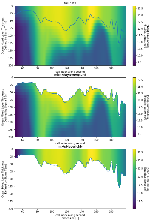
In this case the cell bounds are not available for the model output, but mask_mixedlayer has the option to take those into account and e.g. remove cells only if the lower boundary is within the mixed layer. All you need to do is correctly specify z_bounds with the variable/coordinate name of the cell bounds.

Removing bottom values¶

For similar reasons you might sometimes want to mask out the values closest to the ocean bottom. remove_bottom_values will mask out the bottom-most grid cell at every location.

[42]:

from xarrayutils.utils import remove_bottom_values
ds_bot_removed = remove_bottom_values(ds)
ds_bot_removed

[42]:

<xarray.Dataset>
Dimensions:             (bnds: 2, i: 360, j: 300, lev: 50, member_id: 1, time: 1980, vertices: 4)
Coordinates:
  * i                   (i) int32 0 1 2 3 4 5 6 ... 353 354 355 356 357 358 359
  * j                   (j) int32 0 1 2 3 4 5 6 ... 293 294 295 296 297 298 299
    latitude            (j, i) float64 dask.array<chunksize=(300, 360), meta=np.ndarray>
    longitude           (j, i) float64 dask.array<chunksize=(300, 360), meta=np.ndarray>
  * time                (time) datetime64[ns] 1850-01-16T12:00:00 ... 2014-12...
    time_bnds           (time, bnds) datetime64[ns] dask.array<chunksize=(1980, 2), meta=np.ndarray>
  * member_id           (member_id) <U8 'r1i1p1f1'
  * lev                 (lev) float64 5.0 15.0 25.0 ... 5.499e+03 5.831e+03
    lev_bnds            (lev, bnds) float64 dask.array<chunksize=(50, 2), meta=np.ndarray>
Dimensions without coordinates: bnds, vertices
Data variables:
    mlotst              (member_id, time, j, i, lev) float32 dask.array<chunksize=(1, 196, 300, 360, 50), meta=np.ndarray>
    vertices_latitude   (j, i, vertices, lev) float64 dask.array<chunksize=(300, 360, 4, 50), meta=np.ndarray>
    vertices_longitude  (j, i, vertices, lev) float64 dask.array<chunksize=(300, 360, 4, 50), meta=np.ndarray>
    thetao              (member_id, time, lev, j, i) float32 dask.array<chunksize=(1, 5, 50, 300, 360), meta=np.ndarray>
Attributes:
    grid:                    native atmosphere N96 grid (145x192 latxlon)
    forcing_index:           1
    table_id:                Omon
    variant_label:           r1i1p1f1
    source:                  ACCESS-ESM1.5 (2019): \naerosol: CLASSIC (v1.0)\...
    tracking_id:             hdl:21.14100/4ca9ce2d-6374-4e22-8ad3-1a5a6dfb8fd...
    initialization_index:    1
    physics_index:           1
    run_variant:             forcing: GHG, Oz, SA, Sl, Vl, BC, OC, (GHG = CO2...
    branch_time_in_parent:   21915.0
    history:                 2019-11-15T15:38:06Z ; CMOR rewrote data to be c...
    cmor_version:            3.4.0
    grid_label:              gn
    nominal_resolution:      250 km
    intake_esm_varname:      mlotst\nthetao
    experiment_id:           historical
    realization_index:       1
    parent_activity_id:      CMIP
    sub_experiment_id:       none
    source_id:               ACCESS-ESM1-5
    branch_time_in_child:    0.0
    parent_experiment_id:    piControl
    activity_id:             CMIP
    data_specs_version:      01.00.30
    realm:                   ocean
    product:                 model-output
    Conventions:             CF-1.7 CMIP-6.2
    experiment:              all-forcing simulation of the recent past
    mip_era:                 CMIP6
    institution:             Commonwealth Scientific and Industrial Research ...
    branch_method:           standard
    frequency:               mon
    institution_id:          CSIRO
    title:                   ACCESS-ESM1-5 output prepared for CMIP6
    table_info:              Creation Date:(30 April 2019) MD5:e14f55f257ccea...
    parent_variant_label:    r1i1p1f1
    parent_mip_era:          CMIP6
    parent_time_units:       days since 0101-1-1
    further_info_url:        https://furtherinfo.es-doc.org/CMIP6.CSIRO.ACCES...
    sub_experiment:          none
    source_type:             AOGCM
    version:                 v20191115
    parent_source_id:        ACCESS-ESM1-5
    license:                 CMIP6 model data produced by CSIRO is licensed u...
    intake_esm_dataset_key:  CMIP.CSIRO.ACCESS-ESM1-5.historical.Omon.gn

xarray.Dataset

Dimensions:
- bnds: 2
- i: 360
- j: 300
- lev: 50
- member_id: 1
- time: 1980
- vertices: 4

Coordinates: (9)

i
(i)
int32
0 1 2 3 4 5 ... 355 356 357 358 359
long_name :
cell index along first dimension
units :
1
```
array([  0,   1,   2, ..., 357, 358, 359], dtype=int32)
```
j
(j)
int32
0 1 2 3 4 5 ... 295 296 297 298 299
long_name :
cell index along second dimension
units :
1
```
array([  0,   1,   2, ..., 297, 298, 299], dtype=int32)
```

latitude

(j, i)

float64

dask.array<chunksize=(300, 360), meta=np.ndarray>

bounds :: vertices_latitude
long_name :: latitude
standard_name :: latitude
units :: degrees_north

	Array	Chunk
Bytes	864.00 kB	864.00 kB
Shape	(300, 360)	(300, 360)
Count	5 Tasks	1 Chunks
Type	float64	numpy.ndarray

longitude

(j, i)

float64

dask.array<chunksize=(300, 360), meta=np.ndarray>

bounds :: vertices_longitude
long_name :: longitude
standard_name :: longitude
units :: degrees_east

	Array	Chunk
Bytes	864.00 kB	864.00 kB
Shape	(300, 360)	(300, 360)
Count	5 Tasks	1 Chunks
Type	float64	numpy.ndarray

time

(time)

datetime64[ns]

1850-01-16T12:00:00 ... 2014-12-...

axis :: T
bounds :: time_bnds
long_name :: time
standard_name :: time

array(['1850-01-16T12:00:00.000000000', '1850-02-15T00:00:00.000000000',
       '1850-03-16T12:00:00.000000000', ..., '2014-10-16T12:00:00.000000000',
       '2014-11-16T00:00:00.000000000', '2014-12-16T12:00:00.000000000'],
      dtype='datetime64[ns]')

time_bnds

(time, bnds)

datetime64[ns]

dask.array<chunksize=(1980, 2), meta=np.ndarray>

	Array	Chunk
Bytes	31.68 kB	31.68 kB
Shape	(1980, 2)	(1980, 2)
Count	5 Tasks	1 Chunks
Type	datetime64[ns]	numpy.ndarray

member_id
(member_id)
<U8
'r1i1p1f1'
```
array(['r1i1p1f1'], dtype='<U8')
```

lev

(lev)

float64

5.0 15.0 ... 5.499e+03 5.831e+03

axis :: Z
bounds :: lev_bnds
long_name :: ocean depth coordinate
positive :: down
standard_name :: depth
units :: m

array([5.000000e+00, 1.500000e+01, 2.500000e+01, 3.500000e+01, 4.500000e+01,
       5.500000e+01, 6.500000e+01, 7.500000e+01, 8.500000e+01, 9.500000e+01,
       1.050000e+02, 1.150000e+02, 1.250000e+02, 1.350000e+02, 1.450000e+02,
       1.550000e+02, 1.650000e+02, 1.750000e+02, 1.850000e+02, 1.950000e+02,
       2.050000e+02, 2.168468e+02, 2.413490e+02, 2.807807e+02, 3.432505e+02,
       4.273156e+02, 5.367156e+02, 6.654141e+02, 8.127816e+02, 9.690651e+02,
       1.130935e+03, 1.289605e+03, 1.455770e+03, 1.622926e+03, 1.801558e+03,
       1.984855e+03, 2.182905e+03, 2.388417e+03, 2.610935e+03, 2.842564e+03,
       3.092205e+03, 3.351295e+03, 3.628058e+03, 3.913264e+03, 4.214495e+03,
       4.521918e+03, 4.842566e+03, 5.166130e+03, 5.499245e+03, 5.831294e+03])

lev_bnds

(lev, bnds)

float64

dask.array<chunksize=(50, 2), meta=np.ndarray>

	Array	Chunk
Bytes	800 B	800 B
Shape	(50, 2)	(50, 2)
Count	2 Tasks	1 Chunks
Type	float64	numpy.ndarray

Data variables: (4)

mlotst

(member_id, time, j, i, lev)

float32

dask.array<chunksize=(1, 196, 300, 360, 50), meta=np.ndarray>

cell_measures :: area: areacello
cell_methods :: area: mean where sea time: mean
comment :: Sigma T is potential density referenced to ocean surface.
history :: 2019-11-15T15:38:05Z altered by CMOR: replaced missing value flag (-1e+20) with standard missing value (1e+20).
long_name :: Ocean Mixed Layer Thickness Defined by Sigma T
standard_name :: ocean_mixed_layer_thickness_defined_by_sigma_t
units :: m

	Array	Chunk
Bytes	42.77 GB	4.23 GB
Shape	(1, 1980, 300, 360, 50)	(1, 196, 300, 360, 50)
Count	189 Tasks	11 Chunks
Type	float32	numpy.ndarray

vertices_latitude

(j, i, vertices, lev)

float64

dask.array<chunksize=(300, 360, 4, 50), meta=np.ndarray>

units :: degrees_north

	Array	Chunk
Bytes	172.80 MB	172.80 MB
Shape	(300, 360, 4, 50)	(300, 360, 4, 50)
Count	21 Tasks	1 Chunks
Type	float64	numpy.ndarray

vertices_longitude

(j, i, vertices, lev)

float64

dask.array<chunksize=(300, 360, 4, 50), meta=np.ndarray>

units :: degrees_east

	Array	Chunk
Bytes	172.80 MB	172.80 MB
Shape	(300, 360, 4, 50)	(300, 360, 4, 50)
Count	21 Tasks	1 Chunks
Type	float64	numpy.ndarray

thetao

(member_id, time, lev, j, i)

float32

dask.array<chunksize=(1, 5, 50, 300, 360), meta=np.ndarray>

cell_measures :: area: areacello volume: volcello
cell_methods :: area: mean where sea time: mean
comment :: Diagnostic should be contributed even for models using conservative temperature as prognostic field.
long_name :: Sea Water Potential Temperature
standard_name :: sea_water_potential_temperature
units :: degC

	Array	Chunk
Bytes	42.77 GB	108.00 MB
Shape	(1, 1980, 50, 300, 360)	(1, 5, 50, 300, 360)
Count	5546 Tasks	396 Chunks
Type	float32	numpy.ndarray

Attributes: (45)
grid :
native atmosphere N96 grid (145x192 latxlon)
forcing_index :
1
table_id :
Omon
variant_label :
r1i1p1f1
source :
ACCESS-ESM1.5 (2019): aerosol: CLASSIC (v1.0) atmos: HadGAM2 (r1.1, N96; 192 x 145 longitude/latitude; 38 levels; top level 39255 m) atmosChem: none land: CABLE2.4 landIce: none ocean: ACCESS-OM2 (MOM5, tripolar primarily 1deg; 360 x 300 longitude/latitude; 50 levels; top grid cell 0-10 m) ocnBgchem: WOMBAT (same grid as ocean) seaIce: CICE4.1 (same grid as ocean)
tracking_id :
hdl:21.14100/4ca9ce2d-6374-4e22-8ad3-1a5a6dfb8fde hdl:21.14100/5c349831-3686-44bd-a668-b5473685d419 hdl:21.14100/daa38aaf-a8b6-432b-8711-b8e3d73ba87f hdl:21.14100/79363e12-71ec-45ff-8ac7-5d9caaf123be hdl:21.14100/a0ac1b51-fd2a-49b3-ac10-cf7f1afeb09c hdl:21.14100/33ea2626-c182-4510-924f-833bfa6efada hdl:21.14100/20e5ecb1-cbe8-438f-945e-762dfbef1caf hdl:21.14100/115a1ec8-d7c7-44d0-ae29-860faf8daea8 hdl:21.14100/d85fa960-37cc-439f-ad46-acb60581b568 hdl:21.14100/da6b29c5-d498-456f-ac04-63d595d7721e hdl:21.14100/47712943-793d-45ab-acca-b62678bce71b hdl:21.14100/1a06ae50-aac9-4e42-bf90-365ecffa0fd6 hdl:21.14100/42c2ee1a-2dc2-4976-a781-e9ce77da01c1 hdl:21.14100/19003e14-c05a-42bc-87e2-697106b55748 hdl:21.14100/2d3419d6-fc7c-4d65-9e90-ae36411f6627 hdl:21.14100/b292c680-e324-487d-89af-5e95579a6adf hdl:21.14100/5533bdc5-d82b-48ec-acd2-d4f07903f67c hdl:21.14100/c26507e7-0f70-402c-9f87-741919c26350
initialization_index :
1
physics_index :
1
run_variant :
forcing: GHG, Oz, SA, Sl, Vl, BC, OC, (GHG = CO2, N2O, CH4, CFC11, CFC12, CFC113, HCFC22, HFC125, HFC134a)
branch_time_in_parent :
21915.0
history :
2019-11-15T15:38:06Z ; CMOR rewrote data to be consistent with CMIP6, CF-1.7 CMIP-6.2 and CF standards. 2019-11-15T15:08:04Z ; CMOR rewrote data to be consistent with CMIP6, CF-1.7 CMIP-6.2 and CF standards.
cmor_version :
3.4.0
grid_label :
gn
nominal_resolution :
250 km
intake_esm_varname :
mlotst thetao
experiment_id :
historical
realization_index :
1
parent_activity_id :
CMIP
sub_experiment_id :
none
source_id :
ACCESS-ESM1-5
branch_time_in_child :
0.0
parent_experiment_id :
piControl
activity_id :
CMIP
data_specs_version :
01.00.30
realm :
ocean
product :
model-output
Conventions :
CF-1.7 CMIP-6.2
experiment :
all-forcing simulation of the recent past
mip_era :
CMIP6
institution :
Commonwealth Scientific and Industrial Research Organisation, Aspendale, Victoria 3195, Australia
branch_method :
standard
frequency :
mon
institution_id :
CSIRO
title :
ACCESS-ESM1-5 output prepared for CMIP6
table_info :
Creation Date:(30 April 2019) MD5:e14f55f257cceafb2523e41244962371
parent_variant_label :
r1i1p1f1
parent_mip_era :
CMIP6
parent_time_units :
days since 0101-1-1
further_info_url :
https://furtherinfo.es-doc.org/CMIP6.CSIRO.ACCESS-ESM1-5.historical.none.r1i1p1f1
sub_experiment :
none
source_type :
AOGCM
version :
v20191115
parent_source_id :
ACCESS-ESM1-5
license :
CMIP6 model data produced by CSIRO is licensed under a Creative Commons Attribution-ShareAlike 4.0 International License (https://creativecommons.org/licenses/). Consult https://pcmdi.llnl.gov/CMIP6/TermsOfUse for terms of use governing CMIP6 output, including citation requirements and proper acknowledgment. Further information about this data, including some limitations, can be found via the further_info_url (recorded as a global attribute in this file). The data producers and data providers make no warranty, either express or implied, including, but not limited to, warranties of merchantability and fitness for a particular purpose. All liabilities arising from the supply of the information (including any liability arising in negligence) are excluded to the fullest extent permitted by law.
intake_esm_dataset_key :
CMIP.CSIRO.ACCESS-ESM1-5.historical.Omon.gn

[43]:

roi = dict(i=150, time=0, j=slice(50, 100))
plt.figure(figsize=[10, 15])
for di, (data, label) in enumerate(zip([ds, ds_bot_removed], ['full data', 'bottom layer removed'])):
    plt.subplot(2,1,di+1)
    data.thetao.isel(lev=slice(38, -2),**roi).plot(yincrease=False, robust=True)
    plt.title(label)
    plt.grid()

[ ]:

Utilities for large scale climate data analysis¶

Linear regression¶

Correlation maps¶

Hatch sign agreement¶

Masking values in the mixed layer¶

Removing bottom values¶